The explicit formula and bounding analytic rank from above

Wednesday's post gave some detail on how one can numerically evaluate $L_E(s)$, the $L$-function attached to $E$, at any given complex input $s$. This is certainly the first step in determining the analytic rank of $E$ i.e. the order of vanishing of the $L_E(s)$ at the central point $s=1$.

However, we immediately run into two major issues. The first, as mentioned previously, is that we have no proven lower bound on the size of the coefficients of the Taylor expansion of $L_E(s)$ at $s=1$, so we can never truly ascertain if the $n$th derivative there vanishes, or is just undetectibly small.

Today's post focuses on a method that at least partially overcomes the second issue: that evaluating $L_E(s)$ and its derivatives takes at least $O(\sqrt{N})$ time, where $N$ is the conductor of $E$. This means that working with elliptic curve $L$-functions directly becomes computationally infeasible if the curve's conductor is too big.

To see how we can bypass this problem, we'll have to talk about logarithmic derivatives. The logarithmic derivative of a function  $f(s)$ is just
$$ \frac{d}{ds} \log(f(s)) = \frac{f^{\prime}(s)}{f(s)}. $$
Logarithmic derivatives have some nice properties. For one, they turn products into sums: if $f(s) = g(s)h(s)$, then $\frac{f^{\prime}}{f} = \frac{g^{\prime}}{g} + \frac{h^{\prime}}{h}$. Because we can write $L_E(s)$ as an Euler product indexed by the primes, we therefore have that
$$ \frac{L_E^{\prime}}{L_E}(s) = \sum_p \frac{d}{ds} \log\left(\left(1-a_p p^{-s} + \epsilon_p p^{-2s}\right)^{-1}\right).  $$
When you multiply this out, you rather amazingly get a Dirichlet series whose coefficients can be described in a very mathematically elegant way:
$$ \frac{L_E^{\prime}}{L_E}(1+s) = \sum_{n=1}^{\infty} c_n n^{-s}, $$
where
$$ c_n = \begin{cases}
\left(p+1-\#E(\mathbb{F}_{p^m})\right)\frac{\log p}{p^m}, & n = p^m \mbox{a perfect prime power,} \\
0 & \mbox{otherwise.}\end{cases} $$

That is, the $n$th coefficient of $\frac{L_E^{\prime}}{L_E}(1+s)$ is $0$ when $n$ is not a prime power, and when it is, the coefficient relates directly to the number of points on the reduced curve over the finite field of $n$ elements. [Note we're shifting the logarithmic derivative over to the left by one unit, as this puts the central point at the origin i.e. at $s=0$.]

How does this yield a way to estimate analytic rank? Via something called the Explicit Formula for elliptic curve $L$-functions - which, confusingly, is really more of a suite of related methods than any one specific formula.

Remember the Generalized Riemann Hypothesis? This asserts, in the case of elliptic curve $L$-functions at least, that all nontrivial zeros of $L_E(s)$ lie on the line $\Re(s) = 1$, and two zeros can never lie on top of each other except at the central point $s=1$. The number of such zeros at the central point is precisely the analytic rank of $E$. Each nontrivial zero can therefore be written as $1\pm i\gamma$ for some non-negative real value of $\gamma$ - it turns out that whenever $L_E(1+i\gamma)=0$, then $L_E(1-i\gamma)=0$ too, so noncentral zeros always come in pairs. We believe GRH to be true with a high degree of confidence, since in the 150 years that $L$-functions have been studied, no-one has ever found a non-trivial zero off the critical line.

We can invoke GRH with logarithmic derivatives and something called the Hadamard product representation of an entire function to get another formula for the logarithmic derivative of $L_E(s)$:
$$ \frac{L_E^{\prime}}{L_E}(1+s) = -\log\left(\frac{\sqrt{N}}{2\pi}\right) - \frac{\Gamma^{\prime}}{\Gamma}(1+s) + \sum_{\gamma} \frac{s}{s^2+\gamma^2}. $$
Here $\frac{\Gamma^{\prime}}{\Gamma}(s)$ is the logarithmic derivative of the Gamma function (known as the digamma function; this is a standard function in analysis that we know a lot about and can easily compute), and $\gamma$ runs over the imaginary parts of the zeros of $L_E(s)$ on the critical strip $\Re(s)=1$.

What does this get us? A way to equate a certain sum over the zeros of $L_E(s)$ to other more tractable functions and sums. When you combine the two formulae for $\frac{L_E^{\prime}}{L_E}(1+s)$ you get the following equality:

$$ \sum_{\gamma} \frac{s}{s^2+\gamma^2} = \log\left(\frac{\sqrt{N}}{2\pi}\right) + \frac{\Gamma^{\prime}}{\Gamma}(1+s) + \sum_n \frac{c_n}{n} n^{-s}.$$

The key realization here is that while computing the zeros of $L_E$ is in general nontrivial and time-consuming, all the other quantities in the equation above are readily computable. We can therefore evaluate on the left by computing the quantities on the right to sufficient precision, none of which require knowledge of the exact locations of the zeros of $L_E(s)$.

The above is the first and perhaps most basic example of an explicit formula for elliptic curve $L$-functions, but it is not the one we want. Specificially, trouble still arises in the fact that when were still dealing with an infinite sum on the right, and when we look close to the central point $s=0$, convergence is unworkably slow. We can, however, work with related explicit formulae that reduce the sum on the right to a finite one.

The formula we'll use in our code can be obtained from the above equation by dividing both sides by $s^2$ and taking inverse Laplace transforms; we can also formulate it in terms of Fourier transforms. Specifically, we get the following. Recall the sinc function $\mbox{sinc}(x) = \frac{\sin(\pi x)}{\pi x}$ with $\mbox{sinc}(0)=1$. Then we have:
$$ \sum_{\gamma} \mbox{sinc}(\Delta\gamma)^2 = Q(\Delta,N) + \sum_{\log n<2\pi\Delta} c_n\cdot\left(2\pi\Delta-\log n\right), $$
where $Q(\Delta,N)$ is a certain quantity depending only on $\Delta$ and $N$ that is easy to compute.

Let's look at the left hand side. Since $\mbox{sinc}(\Delta\gamma)^2$ is non-negative for any $\gamma$, and $\mbox{sinc}(0)^2 = 1$, when we sum over all zeros $\gamma$'s we get a value which must be strictly greater than the number of zeros at the central point (i.e. the analytic rank of $E$). Moreover, as we increase $\Delta$, the contribution to the sum from all the noncentral zeros goes to zero, as $\mbox{sinc}(x) \to 0$ as $x \to \infty$.

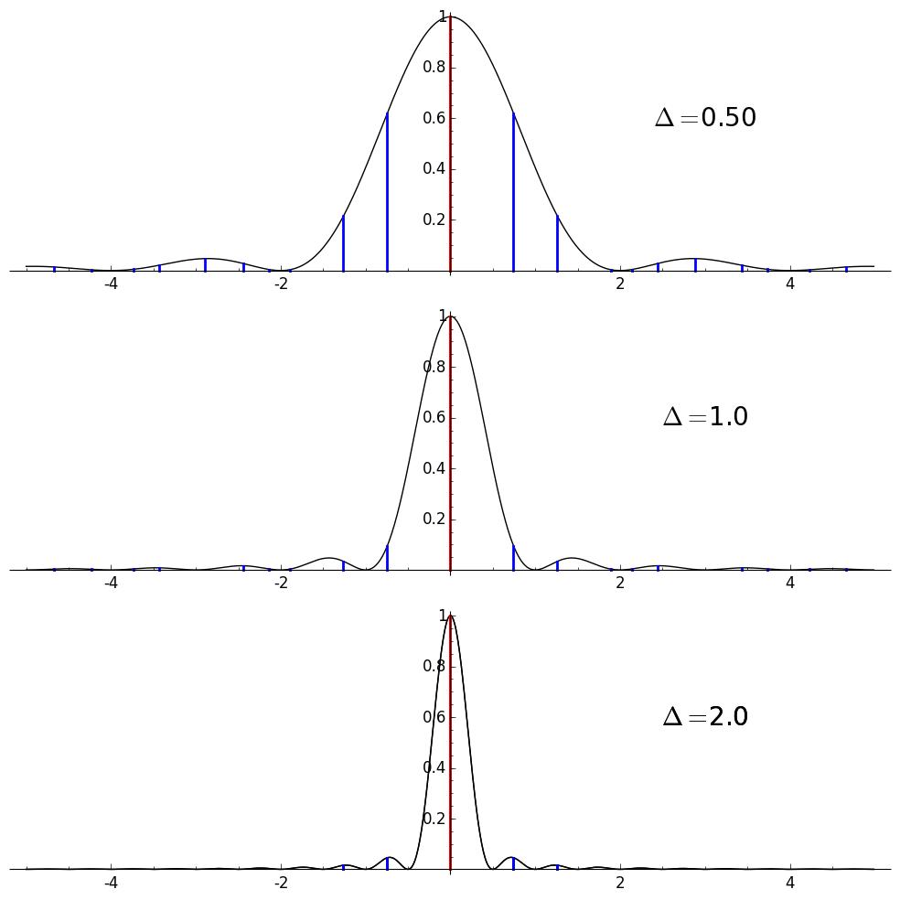
A graphic representation of the sum on the left side of the equation for the $L$-function attached to the elliptic curve $y^2 = x^3 + 103x - 51$ for three increasing values of the parameter $\Delta$. Vertical lines have been plotted at $x=\gamma$ whenever $L_E(1+i\gamma) = 0$, and the height of each line is given by the black curve $\mbox{sinc}(\Delta x)^2$. Thus summing up the length of the vertical lines gives you the value of the sum on the left side of the equation. We see that as $\Delta$ increases, the contribution from the blue lines - corresponding to noncentral zeros - goes to zero, while the contribution from the central zeros in red remain at 1 apiece. Since there are two central zeros (plotted on top of each other here), the sum will limit to 2 from above as $\Delta$ increases.

Now consider the right hand side of the sum. Note that the sum over $n$ is finite, so we can compute it to any given precision without having to worry about truncation error. Since $Q(\Delta,N)$ is easy to compute, this allows us to evaluate the entire right hand side with (relatively) little fuss. We therefore are able, via this equality, to compute a quantity that converges to $r$ from above as $\Delta \to \infty$.

A graphical representation of the finite sum $\sum_{\log n<2\pi\Delta} c_n\cdot\left(2\pi\Delta-\log n\right)$ for the same curve, with $\Delta=1$. The black lines are the triangular function $y = \pm (2\pi\Delta-x)$, whose value at $\log n$ weight the $c_n$ coefficient. Each blue vertical line is placed at $x=\log n$, and has height $c_n\cdot\left(2\pi\Delta-\log n\right)$. Summing up the signed lengths of the blue lines gives the value of the sum over $n$. Note that there are only 120 non-zero terms in this sum when $\Delta=1$, so it is quick to compute.

This formula, and others akin to it, will form the core functionality of the code I will be writing and adapting to include in Sage, as they give us a way to quickly (at least when $\Delta$ is small) show that the analytic rank of a curve can't be too big.

There are some downsides, of course, most notable of which is that the number of terms in the finite sum on the right is exponential in $\Delta$. Tests show that on a laptop one can evaluate the sum in a few milliseconds for $\Delta=1$, a few seconds for $\Delta = 2$, but the computation takes on the order of days when $\Delta=4$. Nevertheless, for the majority of the elliptic curves we'll be looking at, $\Delta$ values of 2 or less will yield rank bounds that are in fact tight, so this method still has much utility.

Another issue that warrants investigation is to analyze just how fast - or slow - the convergence to $r$ will be as a function of increasing $\Delta$; this will allow us to determine what size $\Delta$ we need to pick a priori to get a good estimate out. But this is a topic for a future date; the next post or two will be dedicated toward detailing how I'm implementing this rank estimation functionality in Sage.

How to compute with elliptic curve L-functions and estimate analytic rank

In a previous post I defined what an elliptic curve $L$-function $L_E(s)$ is, and indicated why the behaviour of the function at the central point $s=1$ is of such great interest: the order of vanishing of $L_E(s)$ at $s=1$ is conjecturally precisely equal to the algebraic rank of $E$.

Because this equality is still conjectural, we will cal the former quantity -- then number of derivitaves of $L_E(s)$ that vanish at $s=1$ - the analytic rank of $E$. The topic of this post is to address the question: given an elliptic curve $E$, how do we go about computing its analytic rank?

Before we can hope to answer this question, we need to know how to evaluate $L_E(s)$ itself for any given $s$. In the previous post I gave both the Euler product and Dirichlet series definitions for $L_E(s)$; to jog your memory, here's the Euler product of $L_E(s)$:
$$ L_E(s) = \prod_p \left(1-a_p p^{-s} + \epsilon_p p^{-2s}\right)^{-1}, $$
where the product runs over all prime numbers, $a_p = p+1-\#\{E(\mathbb{F}_p)\}$, and $\epsilon_p = 0$ if $p$ divides the conductor of $E$ and $1$ otherwise. The Dirichlet series is $L_E(s) = \sum_{n}a_n n^{-s}$, which is precisely what you get when you multiply out the Euler product. Note that we are suppresing the dependence on $E$ in both the $a_n$ and $\epsilon_p$ constants.

However, both the Euler product and Dirichlet series representations of $L_E(s)$ will only converge absolutely when the real part of $s$ exceeds $\frac{3}{2}$. Although the Sato-Tate Conjecture (now a theorem, but the name has stuck) implies that the expansions will in fact converge conditionally for $\Re{s}>\frac{1}{2}$, the convergence is so slow that attempting to evaluate $L_E(s)$ near the central point by multiplying or summing enough terms is horribly inefficient. As such, we need a better way to evaluate $L_E(s)$ - and thankfully, such better ways do indeed exit.

Remember how I mentioned in the previous post that $L$-functions obey a very nice symmetry condition? Well, here's that condition exactly: first, we need to define something called the completed $L$-function $\Lambda_E(s)$. This is just $L_E(s)$ multiplied by some extra factors. Specifically,
$$\Lambda_E(s) = N^{\frac{s}{2}}(2\pi)^{-s}\Gamma(s) L_E(s), $$
where $N$ is the conductor of $E$ and $\Gamma(s)$ is the usual Gamma function on $\mathbb{C}$ (the one that gives you $(n-1)!$ when you evaluate it at the positive integer $s=n$).

We can show that $\Lambda_E(s)$ is entire on $\mathbb{C}$; that is, it doesn't have any poles. Moreover, $\Lambda_E(s)$ obeys the glorious symmetry property
$$ \Lambda_E(s) = w_E \Lambda_E(2-s), $$
where $w_E$ is either $1$ or $-1$ and depends on $E$. This is called the functional equation for the $L$-function attached to $E$.

Another way to put it is that shifted completed $L$-function $\Lambda_E(1+s)$ is either an even or an odd function of $s$. Because the factors $N^{\frac{s}{2}}$, $(2\pi)^{-s}$ and $\Gamma(s)$ are all readily computable, this allows us to determine the value of $L_E(s)$ when the real part of $s$ is less than $\frac{1}{2}$.

What's left, then, is to figure out how to efficinetly evaluate $L_E(s)$ in the strip $\frac{1}{2} \le \Re(s) \le \frac{3}{2}$. This is called the critical strip for the $L$-function, and it is here that the behaviour of the function is most interesting.

[Aside: we can, for example, show that $\Lambda_E(1+s)$ is never zero outside of the critical strip. The Generalized Riemann Hypothesis in fact asserts that elliptic curve $L$-functions are only ever zero along the exact center of this strip, the critical line $\Re(s)=1$. We'll get back to the zeros of elliptic curve $L$-functions in a later post.]

To evaluate $\Lambda_E(s)$ in the critical strip, we make use of the modularity of $E$. The modularity theorem states that elliptic curves are modular: for every elliptic curve $E$ over the rationals there exists a weight 2 cuspidal eigenform $f_E$ of level $N$ (where $N$ is precisely the conductor of $E$), such that the $a_n$ of $E$ as defined previously equal the Fourier coefficients of $f_E$. If you haven't studied modular forms before, the crucial piece of knowledge is that there is a natural procedure for constructing $L$-functions from modular forms in such a way that the definition makes sense for all complex inputs $s$, and that the $L$-function attached to the cusp form $f_E$ will exactly equal the elliptic curve $L$-function $L_E(s)$. This is in fact how we show that elliptic curve $L$-functions can be analytically continued to all of $\mathbb{C}$.

The take-away is that via modularity there is an infinite sum representation for $L_E(s)$ which converges absolutely for all $s$. Here it is: define the auxiliary function
$$\lambda_E(s) = \left(\frac{\sqrt{N}}{2\pi}\right)^{s} \sum_{n=1}^\infty a_n n^{-s}\Gamma \left(s,\frac{2\pi}{\sqrt{N}}\cdot n\right), $$
where all the quantities are as defined previously, and $\Gamma(s,x)$ is the upper incomplete Gamma function (note that since $\Gamma(s,x)$ goes to zero exponentially as $x$ goes to infinity, this sum will converge absolutely for any $s$, with rate of convergence scaling with $\sqrt{N}$). Then we have
$$ \Lambda_E(s) = \lambda_E(s) + w_E \lambda_E(2-s). $$
Because we know how to compute incomplete Gamma functions, this gives us a way to evaluate $\Lambda_E(s)$, and thus $L_E(s)$, in the critical strip. The upside with this formula and variations thereof is that it works for any value of $s$ you stick in - including values near $s=1$. Similar formulae exist for the derivatives of $L_E(s)$, so we can in theory compute $L_E^{(n)}(1)$, the $n$th derivative of $L_E(s)$ at the central point, to any degree of accuracy for any $n$.

Thus if we want to compute a curve's analytic rank, what's stopping us from just evaluating successive derivatives of $L_E(s)$ at $s=1$ until we hit one which is not zero?

Two reasons. The first is that there's no way around the fact that you need about $\sqrt{N}$ terms to compute $L_E(s)$ or its derivatives to decent precision. If the conductor of the curve is too big, as is often the case, it takes an inordinate amount of time to simply evaluate the $L$-function near the central point. This makes direct evaluation impractical for all but the smallest-conductor curves -- and for those curves we can usually compute rank via other methods anyway.

The second reason is a more subtle one: how do you tell numerically if the $n$th derivative of $L_E(s)$ at $s=1$ is zero? If you think about it, it's easy to answer this question in one direction only: if you evaluate $L_E^{(n)}(1)$ to some precision and get digits that aren't all zero, then (assuming your code is correct) the $n$th derivative of $L_E(s)$ does not vanish. However, no matter how many digits of precision we compute getting all zeros, the possibility will always remain that the next digit along might not be zero.

In general, there is no numerical way to determine if the value of a black-box complex-valued function at a point is zero, or just really really close to zero. This is why, if you look in the literature, you'll find "methods to estimate analytic rank", but never to compute the quantity exactly. It's impossible to do without extra knowledge. Specifically, we'd need to have some sort of a computable lower bound on the size of the derivatives of $L_E(s)$ at the central. Unfortunately, no such theorems currently exist, so we're stuck with estimating analytic rank for now.

Thankfully, the $\sqrt{N}$-dependence issue is more hopeful. The next post will detail a method that provides good estimates for the analytic rank that scales much more slowly with the curve's conductor.

How to develop for Sage using Sage Math Cloud and Git

I will be using Sage Math Cloud to write all the code for my Google Summer of Code project. The advantage of choosing the cloud-based route should be clear: you don’t need to install or store anything locally, and it frees you up to use any device with a web browser you choose to write code. The downside, as Sage Math Cloud is still new, is that tutorials and how-tos on the setup process in order to do so are a bit lacking. Since I couldn’t find any single unified source on how to do it, I thought I might to create a step-by-step guide on getting set up in Sage Math Cloud to write code in for inclusion in the Sage codebase.

Much of what I've done follows the Git the Hard Way tutorial for Sage development. However, there are significant departures. I recommend reading through that tutorial first; if you do then what follows below will be a piece of cake.

First, you’ll need an account at cloud.sagemath.com. Good news: the whole service is completely free to use, and there’s no annoying back-and-forthing via emailed confirmation links. It’ll take you two minutes tops.

The cloud.sagemath.com homepage.

Your work on your Sage Math Cloud account is project-based; each account can have a large number of projects associated to it. Each project acts like it’s own Linux-based file system inside of which you can create and edit any number of files of any type. Create a project in which you'll house your code.

The project root view, before any files have been created.

Next, you'll want a local installation of Sage. We're going to initiate a local copy of the Sage master repo, as hosted on GitHub. Click New --> Terminal to open up a new terminal window - we'll be doing everything via terminal commands. Then type the following three commands:

~$ git clone git://github.com/sagemath/sage.git

~$ cd sage

~/sage$ make

The first will download a copy of the Sage codebase into the new folder 'sage' (it should appear in the project root directory after the download is complete); the second changes into the directory, and the third initiated the compiling of the Sage source.

Note that the building of Sage usually takes about 3 hours, so get this going and then kick back and take inspiration from this.

While your code is compiling you'll want to make sure you have a GitHub account. If you don't follow the steps there to create one. While not required, hosting any projects on GitHub is highly recommended: it will allow multiple people to work on a project simultaneously, as well as giving you access to sophisticated revision control functionality that will prevent you from accidentally deleting code or data.

GitHub repo creation page.

Create an empty repository - we'll fill it with things later. So long as the repo exists and you know its name you're good to go.

The next thing we'll want to do is register the Sage Trac repository, where all the active tickets are hosted for Sage development. Once you're done creating an empty repo on your GitHub account, go back to your Sage Math Cloud project and wait for Sage to finish building. When this is done, in the terminal window type the following:

~/sage$ git remote add trac git@trac.sagemath.org:sage.git -t master

~/sage$ git remote -v

origin  git://github.com/sagemath/sage.git (fetch)

origin  git://github.com/sagemath/sage.git (push)

trac    git@trac.sagemath.org:sage.git (fetch)

trac    git@trac.sagemath.org:sage.git (push)

The git remote add command registers the Sage trac repo as a remote repository (trac is the name it is registered as locally; you can of course call it anything you want). The git remote -v command simply lists what repos you have now registered. We won't be using Sage trac for now. If you want more practice with trac, see the Git the Hard Way tutorial mentioned previously.

Note the inclusion of the word master in the command above; this means we will only track the master branch of the remote repo. A branch is an instanced copy of the codebase which you can work on and edit without altering other branches. The master branch should be kept pristine, so we will want to create and switch to a new branch. This is accomplished with the git checkout command:

~/sage$ git checkout -b demo

Switched to a new branch 'demo'

~/sage$ git branch

* demo

  master

The -b parameter creates the branch, while checkout switches to that branch. Typing git branch then shows you what branches currently exist locally, as well as the one you're currently on.

We're now in the position to register the demo branch with our fresh repo on GitHub:

~/sage$ git remote add demo https://github.com/haikona/demo.git

~/sage$ git remote -v

demo    https://github.com/haikona/demo.git (fetch)

demo    https://github.com/haikona/demo.git (push)

origin  git://github.com/sagemath/sage.git (fetch)

origin  git://github.com/sagemath/sage.git (push)

trac    git@trac.sagemath.org:sage.git (fetch)

trac    git@trac.sagemath.org:sage.git (push)

And finally, we can push to our repo to sync the local copy therewith. For this you will need your GitHub password - so not just any old Harry can push to your repo.

~/sage$ git push demo demo

Username for 'https://github.com': haikona

Password for 'https://haikona@github.com':

Counting objects: 4, done.

Delta compression using up to 4 threads.

Compressing objects: 100% (2/2), done.

Writing objects: 100% (3/3), 317 bytes | 0 bytes/s, done.

Total 3 (delta 1), reused 0 (delta 0)

To https://github.com/haikona/demo.git

   2b1d88b..21cddb8  demo -> demo

You're now synced and ready to start writing code! From hereon you should be able to follow one of the many tutorials on working with git; the hard part - setting up - is all done.

Mathematical background: elliptic curves and L-functions

Day 1 of my Google Summer of Code project! I will try post updates at least once a week; I thought a good starting point would be to give an introduction to the mathematical objects that this project revolves around. The next post will then give a more detailed description of the project itself, and the structure of the code that I'm going to adapt, write and include in Sage.

To that end, for this post I will assume some  knowledge of elementary number theory, algebra and  complex analysis, but nothing more complicated than that.

Let $E$ be an elliptic curve over the rational numbers. We can think of $E$ as the set of rational solutions $(x,y)$ to a two-variable cubic equation in the form:
$$ E: y^2 = x^3 + Ax + B $$
for some integers $A$ and $B$, along with an extra "point at infinity". An important criterion is that the $E$ be a smooth curve; this translates to the requirement that the discriminant of the curve, given by $-16(4A^3+27B^2)$, is not zero.

One of the natural questions to ask when considering an elliptic curve is "how many rational solutions are there?" It turns out elliptic curves fall in that sweet spot where the answer could be zero, finitely many or infinitely many - and figuring out which is the case is a deeply non-trivial problem.

The rational solutions form an abelian group with a well-defined group operation that can be easily computed. By a theorem of Mordell, the group of rational points on an elliptic curve $E(\mathbb{Q})$ is finitely generated; we can therefore write
$$ E(\mathbb{Q}) \approx T \times \mathbb{Z}^r,$$
where $T$ is a finite group (called the torsion subgroup of $E$), and $r$ is denoted the algebraic rank of $E$.

The elliptic curve group law explained visually: three points in a straight line add to zero; because the point at infinity is the identity element, this means that the sum R of two points P and Q is the reflection about the real axis of the other point on the curve on the straight line connecting P and Q.

Determining the torsion subgroup of $E$ is a relatively straightforward endeavor. By a theorem of Mazur, rational elliptic curves have torsion subgroups that are (non-canonically) isomorphic to one of precisely fifteen possibilities: $\mathbb{Z}/n\mathbb{Z}$ for $n = 1$ through $10$ or $12$; or $\mathbb{Z}/2\mathbb{Z}\oplus \mathbb{Z}/2n\mathbb{Z}$ for $n = 1$ though $4$. Computing the rank $r$ - the number of independent rational points on $E$ - is the hard part, and it is towards this end that this project hopes to contribute.

Perhaps surprisingly, we can translate the algebraic problem of finding rational solutions to $E$ to an analytic one - at least conjecturally. To understand this we'll need to know what an elliptic curve $L$-function is. These are holomorphic functions defined on the whole complex plane that somehow encode a great deal of information about the elliptic curve they're attached to.

The definition goes as follows: for each prime $p$, count the number of solutions to the elliptic curve equation modulo $p$; we'll call this number $N_p(E)$. Then define the number $a_p(E)$ by
$$ a_p(E) = p+1 - N_p(E). $$
Hasse's Theorem states that $a_p(E)$ is always less that $2\sqrt{p}$ in magnitude for any $p$, and the Sato-Tate conjecure (recently proven by Taylor et al) states that for a fixed elliptic curve, the $a_p$ (suitably transformed) are asymptotically distributed in a semi-circular distribution about zero.

Next, for a given $p$ define the local factor $L_p(s)$ to be the function of the complex variable $s$ as follows:
$$ L_p(s) = \left(1-a_p(E)p^{-s} + \epsilon(p)p^{-2s}\right)^{-1}, $$
where $\epsilon(p)$ is 0 if $p$ divides the conductor of $E$, and 1 otherwise.

The conductor of $E$ is a positive integer that encodes the bad reduction of $E$: for a finite list of primes $p$, when we reduce the curve modulo $p$, we don't get a smooth curve but rather a singular one instead. The conductor is just the product of these primes to the first or second power (or in the cases $p=2$ or $3$, up to the eighth and fifth powers respectively). If you're unfamiliar with elliptic curves, the thing to note is that the conductor always divides the discriminant of $E$, namely the quantity $-16(4A^3+27B^2)$ mentioned previously.

Finally we can define the $L$-function attached to $E$:
$$ L_E(s) = \prod_p L_p(s) = \prod_p \left(1-a_p(E)p^{-s} + \epsilon(p)p^{-2s}\right)^{-1}. $$
The above representation of $L_E(s)$ is called the Euler product form of the $L$-function. If we multiply out the terms and use power series inversion we can also write $L_E(s)$ as a Dirichlet series:
$$ L_E(s) = \sum_{n=1}^{\infty} a_n(E) n^{-s}, $$
where for non-prime $n$ the coefficients $a_n$ are defined to be exactly the integers you get when you multiply out the Euler expansion.

If you do some analysis, using Hasse's bound on the size of the $a_p(E)$ and their distribution according to Sato-Tate, one can show that the above to representations only converge absolutely when the real part of $s$ is greater than $\frac{3}{2}$, and conditionally for $\Re(s)>\frac{1}{2}$. However, the modularity theorem states that these elliptic curve $L$-functions can actually be analytically continued to the entire complex plane. That is, for every elliptic curve $L$-function $L_E(s)$ as defined above, there is an entire function on $\mathbb{C}$ which agrees with the Euler product/Dirichlet series definition for $\Re(s)>1$, but is also defined - and readily computable - for all other complex values of $s$. This entire function is what we actually call the $L$-function attached to $E$.

The way we analytically continue $L_E(s)$ yields that the function is highly symmetric about the line $\Re(s)=1$; moreover, because the function is defined by real coefficients $L_E(s)$ also obeys a reflection symmetry along the real axis. The point $s=1$ is in a very real sense therefore the central value for the $L$-function. It thus makes sense to investigate the behaviour of the function around this point.

Because $L_E(s)$ is entire, it has a Taylor expansion at any given point. We can ask what the Taylor expansion of $L_E(s)$ about the point $s=1$ is, for example. One of the central unproven conjectures in modern-day number theory is the Birch and Swinnerton-Dyer Conjecture: that the order of vanishing of the Taylor expansions of $L_E(s)$ about the point $s=1$ is precisely $r$, the algebraic rank of the elliptic curve $E$. That is, if we let $z=s-1$ so that
$$ L_E(s) = c_0 + c_1 z + c_2 z^2 + \ldots $$
is the expansion of $L_E(s)$ about the central point, the BSD conjecture holds that $c_0$ through $c_{r-1}$ are all zero, and $c_r$ is not zero.

The values of three elliptic curve L-functions along the critical line $1+it$ for $-10<=1<=10$. Blue corresponds to the curve $y^2 = x^3 - 13392x - 1080432$, a rank 0 curve, red is that of $y^2 = x^3 - 16x + 16$, a rank 1 curve, and green is $y^2 = x^3 - 3024x + 46224$, a rank 2 curve. Note that close to the origin the graphs look like non-zero constant function, a straight line through the origin and a parabola respectively.

Thus if we can compute the order of vanishing of the elliptic curve $L$-function at the central point, we can at least conjecturally compute the rank of the curve. This converts an algebraic problem into a numerical one, which is perhaps more tractible.

The techniques we'll use to attempt to do this will be the subject of the next blog post. Unfortunately there are still plenty of challenges to this approach - the least of which boils down to: how do you numerically determine if the value of a function is zero, or just really, really close to zero? The short answer is that without theorems to back you up, you can't -- but we can still make considerable progress toward the problem of computing an elliptic curve's rank.

Gotta pay lip service to the other focus point of this blog, yo.

The unit of success of a trip is the Hat, equal to the number of additional pieces of headgear one returns with from said trip. For example, my recently concluded sojourn to South Africa was 2 Hats successful.

Two Weeks Down South

Back from South Africa!

I've just spent a fortnight back in my motherland. I went over for a number of reasons: first and foremost, my US F-1 visa was due to expire soon, so I needed to renew it in order to continue to be able to enter and exit the country while I'm still studying here. While in SA I also voted (the South African national elections were held on May 5) and renewed my pilot's license.

Consequently, very little math or coding has occurred in the past two weeks. So: time to get back in the swing of things! Stay tuned folks.

- Simon