The explicit formula and bounding analytic rank from above

Wednesday's post gave some detail on how one can numerically evaluate $L_E(s)$, the $L$-function attached to $E$, at any given complex input $s$. This is certainly the first step in determining the analytic rank of $E$ i.e. the order of vanishing of the $L_E(s)$ at the central point $s=1$.

However, we immediately run into two major issues. The first, as mentioned previously, is that we have no proven lower bound on the size of the coefficients of the Taylor expansion of $L_E(s)$ at $s=1$, so we can never truly ascertain if the $n$th derivative there vanishes, or is just undetectibly small.

Today's post focuses on a method that at least partially overcomes the second issue: that evaluating $L_E(s)$ and its derivatives takes at least $O(\sqrt{N})$ time, where $N$ is the conductor of $E$. This means that working with elliptic curve $L$-functions directly becomes computationally infeasible if the curve's conductor is too big.

To see how we can bypass this problem, we'll have to talk about logarithmic derivatives. The logarithmic derivative of a function  $f(s)$ is just
$$ \frac{d}{ds} \log(f(s)) = \frac{f^{\prime}(s)}{f(s)}. $$
Logarithmic derivatives have some nice properties. For one, they turn products into sums: if $f(s) = g(s)h(s)$, then $\frac{f^{\prime}}{f} = \frac{g^{\prime}}{g} + \frac{h^{\prime}}{h}$. Because we can write $L_E(s)$ as an Euler product indexed by the primes, we therefore have that
$$ \frac{L_E^{\prime}}{L_E}(s) = \sum_p \frac{d}{ds} \log\left(\left(1-a_p p^{-s} + \epsilon_p p^{-2s}\right)^{-1}\right).  $$
When you multiply this out, you rather amazingly get a Dirichlet series whose coefficients can be described in a very mathematically elegant way:
$$ \frac{L_E^{\prime}}{L_E}(1+s) = \sum_{n=1}^{\infty} c_n n^{-s}, $$
where
$$ c_n = \begin{cases}
\left(p+1-\#E(\mathbb{F}_{p^m})\right)\frac{\log p}{p^m}, & n = p^m \mbox{a perfect prime power,} \\
0 & \mbox{otherwise.}\end{cases} $$

That is, the $n$th coefficient of $\frac{L_E^{\prime}}{L_E}(1+s)$ is $0$ when $n$ is not a prime power, and when it is, the coefficient relates directly to the number of points on the reduced curve over the finite field of $n$ elements. [Note we're shifting the logarithmic derivative over to the left by one unit, as this puts the central point at the origin i.e. at $s=0$.]

How does this yield a way to estimate analytic rank? Via something called the Explicit Formula for elliptic curve $L$-functions - which, confusingly, is really more of a suite of related methods than any one specific formula.

Remember the Generalized Riemann Hypothesis? This asserts, in the case of elliptic curve $L$-functions at least, that all nontrivial zeros of $L_E(s)$ lie on the line $\Re(s) = 1$, and two zeros can never lie on top of each other except at the central point $s=1$. The number of such zeros at the central point is precisely the analytic rank of $E$. Each nontrivial zero can therefore be written as $1\pm i\gamma$ for some non-negative real value of $\gamma$ - it turns out that whenever $L_E(1+i\gamma)=0$, then $L_E(1-i\gamma)=0$ too, so noncentral zeros always come in pairs. We believe GRH to be true with a high degree of confidence, since in the 150 years that $L$-functions have been studied, no-one has ever found a non-trivial zero off the critical line.

We can invoke GRH with logarithmic derivatives and something called the Hadamard product representation of an entire function to get another formula for the logarithmic derivative of $L_E(s)$:
$$ \frac{L_E^{\prime}}{L_E}(1+s) = -\log\left(\frac{\sqrt{N}}{2\pi}\right) - \frac{\Gamma^{\prime}}{\Gamma}(1+s) + \sum_{\gamma} \frac{s}{s^2+\gamma^2}. $$
Here $\frac{\Gamma^{\prime}}{\Gamma}(s)$ is the logarithmic derivative of the Gamma function (known as the digamma function; this is a standard function in analysis that we know a lot about and can easily compute), and $\gamma$ runs over the imaginary parts of the zeros of $L_E(s)$ on the critical strip $\Re(s)=1$.

What does this get us? A way to equate a certain sum over the zeros of $L_E(s)$ to other more tractable functions and sums. When you combine the two formulae for $\frac{L_E^{\prime}}{L_E}(1+s)$ you get the following equality:

$$ \sum_{\gamma} \frac{s}{s^2+\gamma^2} = \log\left(\frac{\sqrt{N}}{2\pi}\right) + \frac{\Gamma^{\prime}}{\Gamma}(1+s) + \sum_n \frac{c_n}{n} n^{-s}.$$

The key realization here is that while computing the zeros of $L_E$ is in general nontrivial and time-consuming, all the other quantities in the equation above are readily computable. We can therefore evaluate on the left by computing the quantities on the right to sufficient precision, none of which require knowledge of the exact locations of the zeros of $L_E(s)$.

The above is the first and perhaps most basic example of an explicit formula for elliptic curve $L$-functions, but it is not the one we want. Specificially, trouble still arises in the fact that when were still dealing with an infinite sum on the right, and when we look close to the central point $s=0$, convergence is unworkably slow. We can, however, work with related explicit formulae that reduce the sum on the right to a finite one.

The formula we'll use in our code can be obtained from the above equation by dividing both sides by $s^2$ and taking inverse Laplace transforms; we can also formulate it in terms of Fourier transforms. Specifically, we get the following. Recall the sinc function $\mbox{sinc}(x) = \frac{\sin(\pi x)}{\pi x}$ with $\mbox{sinc}(0)=1$. Then we have:
$$ \sum_{\gamma} \mbox{sinc}(\Delta\gamma)^2 = Q(\Delta,N) + \sum_{\log n<2\pi\Delta} c_n\cdot\left(2\pi\Delta-\log n\right), $$
where $Q(\Delta,N)$ is a certain quantity depending only on $\Delta$ and $N$ that is easy to compute.

Let's look at the left hand side. Since $\mbox{sinc}(\Delta\gamma)^2$ is non-negative for any $\gamma$, and $\mbox{sinc}(0)^2 = 1$, when we sum over all zeros $\gamma$'s we get a value which must be strictly greater than the number of zeros at the central point (i.e. the analytic rank of $E$). Moreover, as we increase $\Delta$, the contribution to the sum from all the noncentral zeros goes to zero, as $\mbox{sinc}(x) \to 0$ as $x \to \infty$.

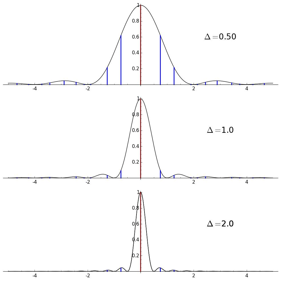A graphic representation of the sum on the left side of the equation for the $L$-function attached to the elliptic curve $y^2 = x^3 + 103x - 51$ for three increasing values of the parameter $\Delta$. Vertical lines have been plotted at $x=\gamma$ whenever $L_E(1+i\gamma) = 0$, and the height of each line is given by the black curve $\mbox{sinc}(\Delta x)^2$. Thus summing up the length of the vertical lines gives you the value of the sum on the left side of the equation. We see that as $\Delta$ increases, the contribution from the blue lines - corresponding to noncentral zeros - goes to zero, while the contribution from the central zeros in red remain at 1 apiece. Since there are two central zeros (plotted on top of each other here), the sum will limit to 2 from above as $\Delta$ increases.

Now consider the right hand side of the sum. Note that the sum over $n$ is finite, so we can compute it to any given precision without having to worry about truncation error. Since $Q(\Delta,N)$ is easy to compute, this allows us to evaluate the entire right hand side with (relatively) little fuss. We therefore are able, via this equality, to compute a quantity that converges to $r$ from above as $\Delta \to \infty$.

A graphical representation of the finite sum $\sum_{\log n<2\pi\Delta} c_n\cdot\left(2\pi\Delta-\log n\right)$ for the same curve, with $\Delta=1$. The black lines are the triangular function $y = \pm (2\pi\Delta-x)$, whose value at $\log n$ weight the $c_n$ coefficient. Each blue vertical line is placed at $x=\log n$, and has height $c_n\cdot\left(2\pi\Delta-\log n\right)$. Summing up the signed lengths of the blue lines gives the value of the sum over $n$. Note that there are only 120 non-zero terms in this sum when $\Delta=1$, so it is quick to compute.

This formula, and others akin to it, will form the core functionality of the code I will be writing and adapting to include in Sage, as they give us a way to quickly (at least when $\Delta$ is small) show that the analytic rank of a curve can't be too big.

There are some downsides, of course, most notable of which is that the number of terms in the finite sum on the right is exponential in $\Delta$. Tests show that on a laptop one can evaluate the sum in a few milliseconds for $\Delta=1$, a few seconds for $\Delta = 2$, but the computation takes on the order of days when $\Delta=4$. Nevertheless, for the majority of the elliptic curves we'll be looking at, $\Delta$ values of 2 or less will yield rank bounds that are in fact tight, so this method still has much utility.

Another issue that warrants investigation is to analyze just how fast - or slow - the convergence to $r$ will be as a function of increasing $\Delta$; this will allow us to determine what size $\Delta$ we need to pick a priori to get a good estimate out. But this is a topic for a future date; the next post or two will be dedicated toward detailing how I'm implementing this rank estimation functionality in Sage.